A Computer Scientist's Guide to Riemannian Manifolds

The main text of this blog is written by hand, with an LLM proofreading the mathematical details and creating some visualizations. Last updated: Oct 6, 2026.

A lot of my CS friends have asked me about various Riemannian manifolds in generative modeling, especially their geometric properties that induce important concepts such as the exponential map and logarithm map used in Riemannian flow matching . Recalling the difficulty I had as a computer science student reading standard mathematics textbooks that run to hundreds of pages, I have been thinking about writing a blog post as a gentle introduction to the basics of Riemannian manifolds and some commonly encountered Riemannian manifolds in machine learning tasks. Currently, I have included the following manifolds: Euclidean Space, Flat Torus, Spherical Manifold, and 3D Rotation Group. You can navigate using the left sidebar for quick reference.

Generally, I will try to avoid using too much mathematical jargon and focus on the intuition behind each concept. Nonetheless, for those who are interested in the mathematical details (like me!), I include them in collapsible sections. Feel free to skip them as the main text is designed to be self-contained. As a self-taught non-mathematician in Riemannian geometry, I will inevitably make some mistakes. Please email me if you find any errors or have any suggestions.

Riemannian Manifold

A manifold $\mathcal{M}$ is a space that locally admits Euclidean coordinates. Imagine you are a tiny ant on the manifold: your immediate surroundings will feel approximately flat, much as we humans do on the spherical Earth. For a smooth manifold, the tangent space $T_x\mathcal{M}$ at a specific point $x\in\mathcal{M}$ can be understood as the vector space of all possible directions (i.e., tangent vectors) in which one can move from $x$. The tangent bundle $T\mathcal{M}:=\bigcup_{x\in \mathcal{M}}(\{x\}\times T_x\mathcal{M})$ is defined as the disjoint union of all tangent spaces at each point. See for an illustration of the tangent space.

Tangent bundle

Including the base point $x$ in the disjoint union is important for manifolds that can be embedded in $\mathbb{R}^m$, whose tangent spaces are $n$-dimensional linear subspaces that may intersect each other. Mathematicians call this a fiber bundle, where each tangent space is called a fiber.

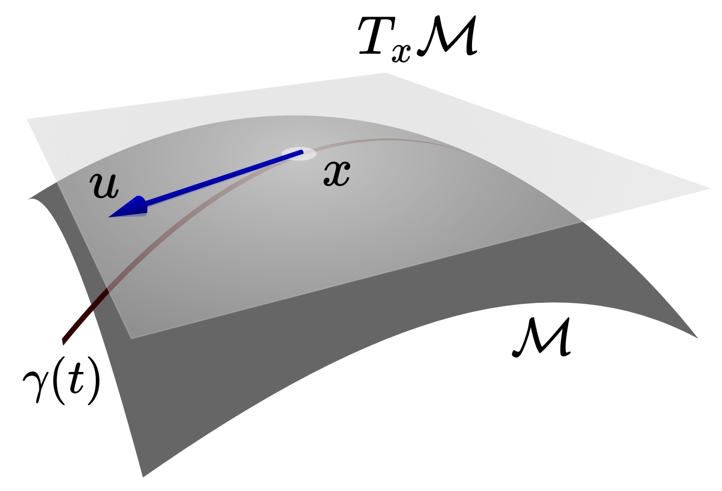
Tangent vector $u\in T_x\mathcal{M}$ at $x\in\mathcal{M}$ along the geodesic $\gamma$.

A Riemannian manifold $\mathcal{M}$ is a smooth manifold equipped with a Riemannian metric $g$, which is a smooth positive-definite inner product on the tangent space of each point: $\begin{equation} g_x: T_x\mathcal{M}\times T_x\mathcal{M}\to \mathbb{R}. \end{equation}$ As $g$ is an inner product, we also write $\langle u,v\rangle_g:=g(u,v)$ and sometimes omit the subscript $x$ if it can be inferred from the context. However, it is important to keep in mind that the Riemannian metric depends on the point. The Riemannian norm of a tangent vector $u\in T_x\mathcal{M}$ is defined as $\|u\|_g:=\sqrt{\langle u,u\rangle_g}$. In this way, the Riemannian metric allows us to define the length of tangent vectors, which is essential for defining the distance between two points on the manifold. Recall from calculus that the infinitesimal arc length of a smooth curve is $\mathrm{d}s=\|f^\prime(t)\|_2\,\mathrm{d}t$ for a smooth curve $f:[0,T]\to\mathbb{R}^n$. The infinitesimal arc length of a smooth curve $\gamma:[0,T]\to\mathcal{M}$ on the Riemannian manifold can be calculated as: $\begin{equation} \mathrm{d}s=\|\dot\gamma(t)\|_g\,\mathrm{d}t=\sqrt{\langle\dot\gamma(t),\dot\gamma(t)\rangle_g}\,\mathrm{d}t. \end{equation}$ Here, we follow the convention of using Newton’s notation to denote derivatives with respect to $t$.

Geodesic, Exponential Map & Logarithm Map

In Euclidean geometry, one specific family of curves is crucial to the standard geometry: the straight lines. On a Riemannian manifold, we naturally want to extend the idea of straight lines to curved spaces. Imagine driving a car on a curved surface with its steering held straight: the route you trace is a straight line on the manifold, known as a geodesic.

One fundamental result for geodesics is the local existence and uniqueness theorem, which states that for any point $x\in\mathcal{M}$ and any tangent vector $u\in T_x\mathcal{M}$, there exists a unique geodesic $\gamma:[0,T]\to\mathcal{M}$ such that $\gamma(0)=x$ and $\dot\gamma(0)=u$. There are some interesting properties of geodesics as the straight lines on the Riemannian manifold. One frequently mentioned property is that a geodesic is a locally distance-minimizing curve. This can be understood as the generalization of the well-known result from elementary school that, in the Euclidean space, the shortest path between two points is the straight line segment. This property can also be understood in terms of kinetic-energy minimization, with the energy functional defined as: $\begin{equation} E(\gamma)=\frac{1}{2}\int_0^Tg_{\gamma(t)}(\dot\gamma(t),\dot\gamma(t))\,\mathrm{d}t. \end{equation}$ Using classical techniques from the calculus of variations, one can derive the geodesic equation for explicitly solving the geodesic $\gamma(t)$, which we will omit here. The geodesic distance $d_g(x,y)$ between two points $x,y\in\mathcal{M}$ is defined as the length of the globally length-minimizing curve that connects $x$ and $y$The four main examples below are complete and connected, so minimizing geodesics exist.. As a global optimum is also a local optimum, the geodesic distance is always the curve length of some geodesic. However, the converse is not necessarily true, i.e., the curve length of a geodesic connecting two points is not necessarily the geodesic distance.

Length-minimizing property

One common misunderstanding is that the geodesic is the globally shortest path between any two points on the manifold. This is not true in general. For example, consider the sphere whose geodesics are the great circles. For a pair of non-antipodal points, the great circle is cut into a shorter arc and a longer arc, both of which are geodesics. However, only the shorter path is the globally shortest path. Another example is provided below. A globally minimizing geodesic exists under the completeness and connectedness assumptions above.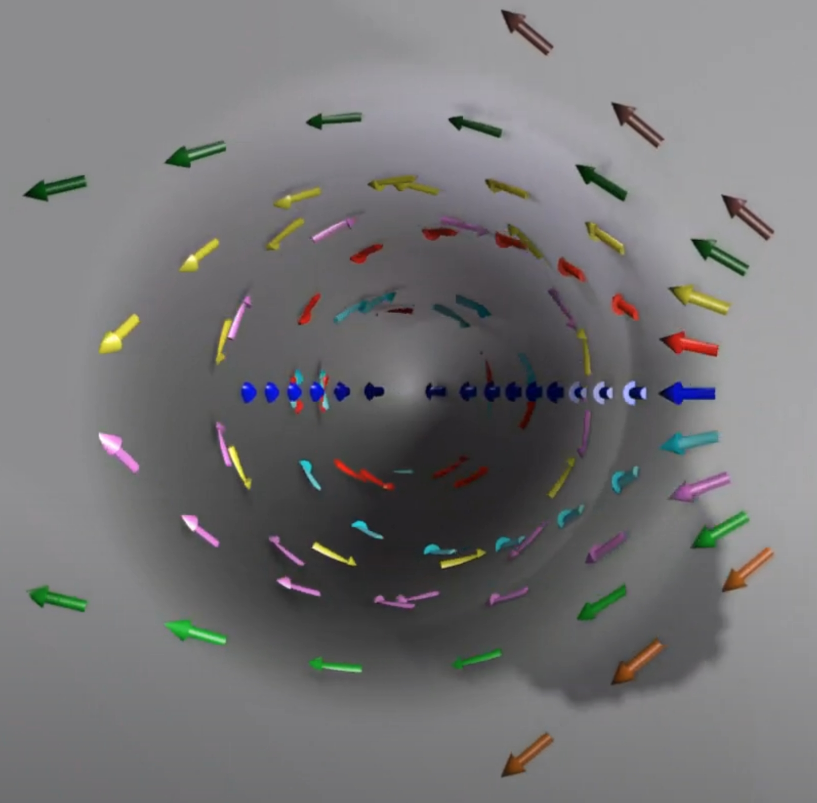

Example showing that the geodesic is not necessarily a globally distance-minimizing curve. Starting from the same point on one side of a steep hill, the geodesics reach the other side by different routes. The blue geodesic that climbs up the hill is longer than the green ones that go around the hill to reach the other side. Figure from Eugene Khutoryansky's video.

More general definition

While other standard approaches derive geodesics from the locally length-minimizing property, we could adopt the kinematic definition in which the velocity remains parallel along the curve. It turns out that the definition of constant tangent vectors is non-trivial, as the tangent spaces are different for different points. Formally, a geodesic is defined by an affine connection $\nabla$ such that $\nabla_{\dot\gamma}\dot\gamma=0$ defines the concept of constant, leading to the general definition of affine geodesic. For general affine geodesics, the locally length-minimizing property no longer holds. In contrast, the standard locally length-minimizing geodesic is a special case of the affine geodesic, which is known as the Levi-Civita geodesic. The Levi-Civita geometry is uniquely defined by the Riemannian metric and is therefore also referred to as the canonical Riemannian structure.

The exponential map $\exp:T\mathcal{M}\to \mathcal{M}$ answers the question: after traveling for a unit time with constant direction and speed, which point will you reach on the manifold? Formally, for a point $x\in\mathcal{M}$ and a tangent vector $u\in T_x\mathcal{M}$, the exponential map is defined as: $\begin{equation} \exp_x(u):=\gamma(1), \end{equation}$ where $\gamma$ is the unique geodesic that satisfies $\gamma(0)=x$ and $\dot\gamma(0)=u$. The logarithm map assigns a chosen inverse $\log_x(y)\in T_x\mathcal{M}$ of the exponential map, which answers the question: given two points on the manifold, in which direction and how far must one travel to reach one point from the other? Formally, for two points $x,y\in\mathcal{M}$, a chosen logarithm satisfies the following identity on its domain: $\begin{equation} \exp_x(\log_x y)\equiv y . \end{equation}$

Some caveats

On an incomplete manifold, a geodesic may cease to exist before $t=1$, so the exponential map need not be defined for every tangent vector. Scaling the vector down extends the available time but changes the input.
The global uniqueness of a geodesic between any two points on the manifold is not guaranteed. For example, consider a pair of antipodal points on $S^2$: infinitely many semicircular arcs connect them with the same length. In this scenario, the logarithm map is not unique.

Based on the idea of constant speed kinematics, we have $\|\dot\gamma(t)\|_g\equiv\|\dot\gamma(0)\|_g=\|u\|_g$. In this scenario, we have $\begin{equation} \|\log_x (y)\|_g=L(\gamma_{x,y}), \end{equation}$ where $L(\gamma_{x,y})$ is the length of the geodesic $\gamma_{x,y}$ that connects $x$ and $y$. If the chosen logarithm follows a minimizing geodesic, we further have $\|\log_x (y)\|_g=d_g(x,y)$. Similarly, the geodesic interpolation between two points $x,y\in\mathcal{M}$ is defined as $\gamma_{x,y}(t)$ for $t\in[0,1]$. Using the exponential and logarithm maps, the geodesic interpolation can be compactly written as: $\begin{equation} \gamma(t)=\exp_x(t\log_x y). \end{equation}$

When does the assumption hold?

For the canonical Riemannian structure induced by the Levi-Civita connection, the assumption $\|\dot\gamma(t)\|_g\equiv\|\dot\gamma(0)\|_g$ always holds. For a general affine connection, it is not guaranteed. In most cases, we work with the canonical Riemannian structure in this post.

The Riemannian norm and geodesic interpolation are crucial concepts in Riemannian flow matching, in which the probability paths are defined along the geodesics. In the following sections, I will explore some commonly encountered Riemannian manifolds in machine learning tasks.

Euclidean Space

Since Riemannian manifolds generalize Euclidean space $\mathbb{R}^n$, we should first check that their geometry agrees with our familiar Euclidean intuition. The Riemannian metric is the standard Euclidean inner product: $\begin{equation} g_x(u,v)=\langle u,v\rangle=\sum_{i=1}^n u_i v_i. \end{equation}$ Similarly, the Riemannian norm is the standard Euclidean norm $\|\cdot\|_2$. As we can travel in the Euclidean space without obstacles, the exponential map in Euclidean space simply translates the base point by the tangent vector. The exponential and logarithm maps, therefore, can be easily computed as: $\begin{align} \exp_x(u)&=x+u,\\ \log_x(y)&=y-x. \end{align}$

Therefore, geodesic interpolation is linear interpolation between two points: $\begin{equation} \gamma(t)=(1-t)x+ty. \end{equation}$

Wait ... How about the exponential function?

If you came up with this question, then you are probably a math enthusiast! The Euclidean exponential map is affine in $u$, whereas the standard exponential function is $\exp u=e^u$. Wait! We’ve got a conflict even in Euclidean space!

It turns out that we need to consider an alternative Riemannian manifold to resolve this conflict. Consider the manifold of positive real numbers $\mathbb{R}_+$. At each point $x\in\mathbb{R}_+$, the tangent space is identified with $T_x\mathbb{R}_+\cong\mathbb{R}$. We can use the Riemannian metric: $\begin{equation} g_x(u,v)=\frac{uv}{x^2},\quad x\in \mathbb{R}_+,u,v\in T_x\mathbb{R}_+. \end{equation}$ We now verify that the following geodesic $\begin{equation} \gamma(t)=e^{ut} \end{equation}$ satisfies the constant speed requirement with the initial conditions $\gamma(0)=1,\dot\gamma(0)=u$. We first note that $\dot\gamma(t)=u e^{ut}=u\gamma(t)$, which satisfies the initial condition. Calculating the Riemannian norm, we have: $\begin{equation} g_{\gamma(t)}(\dot\gamma(t),\dot\gamma(t))=g_{\gamma(t)}(u\gamma(t),u\gamma(t))=\frac{u^2\gamma(t)^2}{\gamma(t)^2}=u^2. \end{equation}$ In this way, we always have $\|\dot\gamma(t)\|^2_g=u^2$, which is independent of the time $t$. To see directly that it is a geodesic, use the coordinate $z=\log x$: the metric becomes $\mathrm{d}z^2$ and the curve becomes the straight line $z(t)=ut$. Setting $t=1$ recovers the exponential map as $\exp_1(u)=e^u$, which coincides with the standard exponential function.

Why this metric?

You probably wonder why we are using such a seemingly exotic Riemannian metric on $\mathbb{R}_+$. The major reason is that this metric is invariant under scaling: $\begin{equation} g_{\lambda x}(\lambda u,\lambda v)=g_x(u,v),\quad \lambda>0,\ x\in\mathbb{R}_+,\ u,v\in T_x\mathbb{R}_+. \end{equation}$ For the multiplication group, this requirement is natural: scaling with a constant should not affect the geometry. In other words, we are essentially using the logarithmic coordinates to represent the positive real numbers. Therefore, at each point $x\in\mathbb{R}_+$, the tangent vector in logarithmic coordinates is $u/x$, which represents the relative scaling under the group operation of multiplication and also leads to the bi-invariant metric.

We will cover more about such an “invariance” in our later discussion on the Lie group and Lie algebra when discussing the geometry for $\mathrm{SO}(3)$.

Alternative interpretation

We can also provide an alternative interpretation to resolve the conflict between the exponential map and the exponential function by considering general affine geodesics with the same canonical Euclidean metric $\mathrm{d}x^2$ on $\mathbb{R}^+$. Recall that affine geodesics have parallel velocity with respect to a chosen connection. Let’s fix our start point to $x=1$ and consider the tangent vector $u\in\mathbb{R}$. Now consider two rules for parallel velocity:

The coordinate velocity $\dot\gamma$ remains constant.
The relative velocity $\dot\gamma/\gamma=u$ remains constant.

The second rule uses a different affine connection; its Euclidean speed generally varies. The first definition gives the following differential equation: $\begin{equation} \frac{\mathrm{d}}{\mathrm{d}t}\dot\gamma(t)=0,\quad \gamma(0)=1, \dot\gamma(0)=u, \end{equation}$ which gives the solution $\gamma(t)=1+ut$ and the exponential map $\exp_1(u)=1+u$ for $u>-1$. The second definition gives the following differential equation: $\begin{equation} \frac{\mathrm{d}}{\mathrm{d}t}\left(\frac{\dot \gamma(t)}{\gamma(t)}\right)=0,\quad \gamma(0)=1, \dot\gamma(0)=u, \end{equation}$ which gives the solution $\gamma(t)=e^{ut}$ and the exponential map $\exp_1(u)=e^u$. This indicates that the exponential function can also be interpreted as the exponential map of a different affine connection even if the metric itself remains unchanged.

Flat Torus

We now continue to explore the flat torus $\mathbb{T}^n$. For simplicity and better visualization, let’s first consider $n=2$, which is often visualized as a doughnut embedded in three-dimensional Euclidean space. This, however, is actually not an accurate representation when we consider its geometric properties. As its name indicates, a flat torus has zero Gaussian curvature everywhere, meaning its intrinsic geometry is flat just like a Euclidean space. In contrast, the embedded 2D torus has nonzero Gaussian curvature at some points. One can easily roll a flat sheet of paper into a cylinder, which also has zero curvature, but it is impossible to further roll the cylinder into a doughnut without stretching or squeezing the paper.

Therefore, it is better to understand a flat torus as a quotient space of the Euclidean space $\mathbb{R}^n$ by the orthogonal lattice $\mathbb{Z}^n$ as $\mathbb{T}^n=\mathbb{R}^n/\mathbb{Z}^n$. In other words, in the 2D case, we consider the following equivalence relation, identifying points that differ by integer translations in two independent directions: $\begin{equation} (x,y)\sim (x+m,y+n),\quad m,n\in\mathbb{Z}. \end{equation}$ Such an identification can be understood visually as gluing opposite sides of a square in the same direction, as demonstrated in . Crystal structures provide another example for understanding the flat torus. In crystallography, the crystal structure is often represented as a unit cell, the smallest repeating unit. With periodic boundary conditions, the cubic unit cell can be extended to the whole crystal structure. This cubic unit cell is essentially a 3D flat torus.

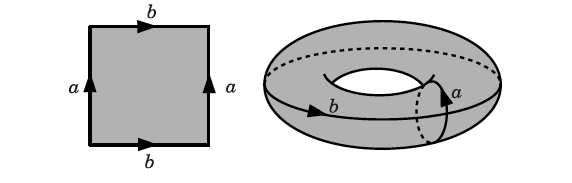
A flat 2D torus constructed by identifying the opposite sides of a square (flat torus), and an embedded 2D torus in three-dimensional Euclidean space as a doughnut-shaped manifold (non-flat torus).

It is also possible to define the quotient space with respect to other values, such as the cell length of a cubic unit cell, or $2\pi$ for a torsion angle, since a rotation of $2\pi$ is equivalent to no rotation. Nonetheless, it is simpler to use fractional coordinates so that each coordinate lies in $[0, 1)$. We will use this unit-period convention in the following discussion, with the standard Euclidean metric and lengths measured in unit-cell units.

About the different tori

We distinguish the flat torus from the embedded torus because we care about their geometric properties in differential geometry. If we consider their topological properties, these two tori are indeed equivalent (more precisely, they are homeomorphic). Homeomorphism allows us to bend and stretch manifolds when establishing equivalence.

At each point $x$ of the flat torus, the tangent space is naturally identified with $T_x\mathbb{T}^n\cong\mathbb{R}^n$. The torus inherits the Euclidean metric and thus the Euclidean 2-norm. Therefore, standard straight lines remain geodesics on flat tori. The exponential map and our default logarithm representative can be computed as:

\begin{align} \exp_x(u)&=(x+u)\bmod 1,\\ \log_x(y)&=(y-x)\bmod 1. \end{align}

Here, modulo is applied componentwise. For the logarithm, any vector $y-x+k$, with $k\in\mathbb{Z}^n$, recovers the same endpoint under the exponential map. We retain the principal-value convention $\log_x(y)\in[0,1)^n$. Additionally, for the different setups of regressing clean data and vector fields in flow matching, we need to be careful about the regression target such that it follows the shortest path for efficient learning.

Regression target in flow matching

The principal-value convention does not guarantee that the learning target follows the shortest path. When the learning target is the clean data, the geodesic distance that follows the shortest path should be used. For example, a prediction $y=0.9$ against the ground truth $x=0.1$ should have a distance loss of $0.2^2$ instead of $0.8^2$ that corresponds to the $\|\log_x y\|_2^2$. This way, the gradient of the loss increases the prediction so it follows the shortest path to the ground truth. For representatives $x,y\in[0,1)^n$, the geodesic distance is: $\begin{equation} d_\mathbb{T}(x,y)=\|\min\{|x-y|,1-|x-y|\}\|_2,\label{eqn:torus_dist} \end{equation}$ where the absolute value and minimum are applied componentwise. In this way, the clean data regression loss is: $\begin{equation} \mathcal{L}_x=d^2_\mathbb{T}(x,y). \end{equation}$

Alternatively, when directly regressing the vector field, the scenario is slightly different. For a ground truth tangent vector $u=0.1$ after applying the principal value convention, a prediction $v=0.9$ should also have a loss of $0.2^2$ instead of $0.8^2$, although both $\|u-v\|_2^2$ and $\|v-u\|_2^2$ give the latter. Similar to the clean data prediction where the tangent vector $x-y$ is wrapped to the shortest one, we additionally require the difference between tangent vectors to be wrapped to the shortest one for vector field regression. Reusing the notation in Eq. \eqref{eqn:torus_dist}, the vector field regression loss is: $\begin{equation} \mathcal{L}_v=d^2_\mathbb{T}(u,v). \end{equation}$

Such conventions are known as the minimum image convention.

Alternative parameterization

For torsion angles with period $2\pi$, using the flat torus $\mathbb{T}_{2\pi}^n=\mathbb{R}^n/(2\pi\mathbb{Z})^n$ is a more intuitive parameterization. In this convention, $x$ and $y$ are angular positions, and tangent components are expressed in radians. With the standard Euclidean metric in these angular coordinates, the tangent norm is $\|u\|_2$. The maps are: $\begin{align} \exp_x(u)&=(x+u)\bmod(2\pi),\\ \log_x(y)&=\operatorname{atan2}(\sin(y-x),\cos(y-x)). \end{align}$

All operations are componentwise. Here, $\operatorname{atan2}$ instead selects the principal logarithm value in $(-\pi,\pi]^n$, following the minimum image convention with a sign choice at half-periods. Changing to this standard angular metric scales lengths by $2\pi$ relative to the unit-period metric above. Similar to previous discussions, the differences between angles and vector fields need to be wrapped for flow matching.

Spherical Manifold

The previous two manifolds are flat manifolds with relatively intuitive and simple geometries. We now move to the spherical manifold $S^n=\{x\in\mathbb{R}^{n+1}:\|x\|_2=1\}$. $S^n$ is an $n$-dimensional manifold embedded in the $(n+1)$-dimensional Euclidean space. As its name indicates, we often visualize $S^2$ as a sphere, the surface of a 3D ball (see ).

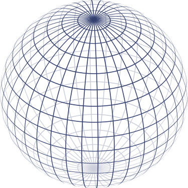
2-sphere embedded in the 3D Euclidean space.

Intuitively, the tangent space at a point $x\in S^n$ on the sphere can be identified as the hyperplane perpendicular to the vector $x$: $T_xS^n=\{u:\langle u,x\rangle=0\}$. As an embedded manifold, $S^n$ inherits the ambient Euclidean metric. Therefore, the spherical metric is exactly the same as the Euclidean one: $g_x(u,v)=\langle u,v\rangle.$

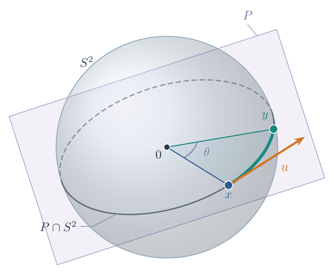
By definition, the geodesic distance between two points $x,y\in S^n$ is the length of the shortest curve connecting them along the sphere. This curve follows the shorter arc of a great circle, obtained by intersecting the sphere with a 2D plane through its center (see ). As the sphere has unit radius, the arc length is exactly the angle between $x$ and $y$, measured in radians: $\begin{equation} d_S(x,y)=\theta:=\arccos\langle x,y\rangle,\quad \theta\in[0,\pi]. \end{equation}$

For example, two perpendicular unit vectors are separated by a distance of $\pi/2$, while two opposite points are separated by $\pi$. In the latter case, there are multiple shortest arcs, all with the same length. The exponential map moves along a great circle in the direction of a tangent vector $u\in T_xS^n$. Using 2D geometry, we obtain: $\begin{equation} \exp_x(u)=x\cos\|u\|_2+\frac{\sin \|u\|_2}{\|u\|_2}u.\label{eqn:sphere_exp} \end{equation}$ As before, the length of $u$ determines how far we travel in one unit of time; on the unit sphere, it also determines the angle through which we rotate.

The plane $P=\operatorname{span}\{x,u\}$ intersects $S^2$ in a great circle. The exponential map $y=\exp_x(u)$ follows this great circle with the arc length $\theta=\|u\|$ for the unit sphere.

Obtaining the exponential map with 2D geometry

For any dimension $n\geq 2$, we can focus on the 2D plane spanned by $x$ and a nonzero tangent vector $u$. Since $\langle x,u\rangle=0$, the vectors $x$ and $v:=u/\|u\|_2$ form an orthonormal basis of this plane. Its intersection with the sphere is a unit circle, and the starting point $x$ has coordinates $(1,0)$ in this basis.

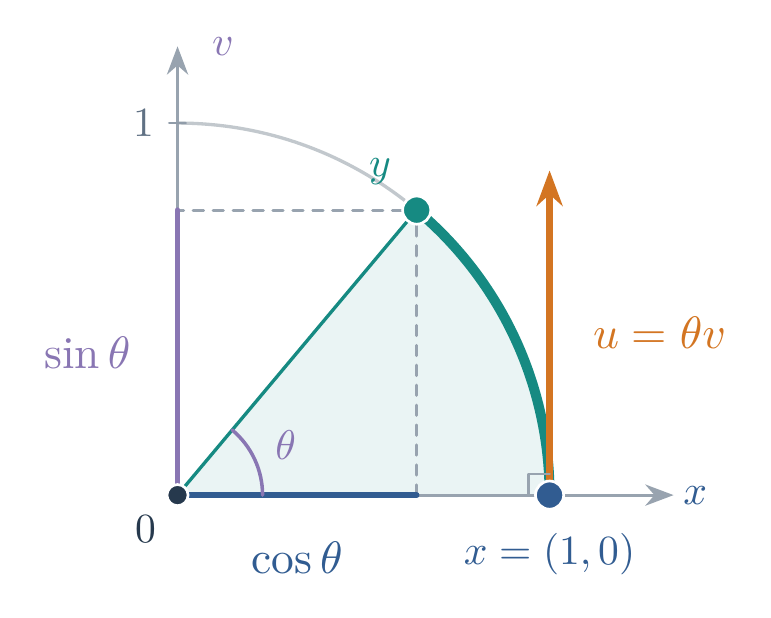
First-quadrant view in the x and v basis, showing the sector angle theta, the tangent vector u, and the cosine and sine projections of y. — The same great circle in the orthonormal basis $(x,v)$, with $v=u/\|u\|_2$. The endpoint $y$ has coordinates $(\cos\theta,\sin\theta)$, giving $y=x\cos\theta+v\sin\theta$.

Now recall that an angle of one radian sweeps out an arc of length one on a unit circle. To travel at speed $\theta=\|u\|_2$, we therefore increase the angle at a rate of $\theta$. At time $t$, the point has 2D coordinates $(\cos(t\theta),\sin(t\theta))$.

To obtain its coordinates in the original Euclidean space $\mathbb{R}^{n+1}$, we resolve these two components along the basis vectors $x$ and $v$:

\begin{equation} \begin{aligned} \gamma(t)&=x\cos(t\theta)+\sin(t\theta)v\\ &=x\cos(t\theta)+\sin(t\theta)\frac{u}{\|u\|_2}. \end{aligned} \end{equation}

Evaluating at $t=1$ gives the exponential map above. This expression remains valid even when $\theta>\pi$, although the arc we travel then goes beyond half a circle and is no longer a shortest path to its endpoint.

Conversely, the logarithm map gives the initial tangent vector that reaches $y$ along the shortest arc from $x$, which amounts to finding the appropriate tangent direction in the 2D plane. Its expression is:

$\begin{equation} \log_x(y)=\frac{\theta}{\sin\theta}(y-\langle x,y\rangle x)=\frac{\arccos\langle x,y\rangle}{\sqrt{1-\langle x,y\rangle^2}}(y-\langle x,y\rangle x), \end{equation}$ where $\theta=\arccos\langle x,y\rangle\in(0,\pi)$.

Obtaining the logarithm map with 2D geometry

In the 2D intersection, it is easy to see that the vector $y-\langle x,y\rangle x$ is the projection of $y$ onto the tangent space at $x$. It points toward $y$ along the great circle and has length $\sin\theta$. Dividing by this length gives a unit direction, and multiplying by $\theta$ gives the required travel distance. This choice of the logarithm is called the principal logarithm, as it selects the shortest arc.

In practice, we also need to handle different numerical stability issues when we implement the spherical manifold with PyTorch (see the discussion below). A detailed standalone implementation can be found in my codebase.

Numerical stability

The following numerical stability issues must be handled when implementing these maps in PyTorch:

The exponential formula is numerically unstable at $u\approx0$. Use torch.sinc(theta / torch.pi) (PyTorch uses the normalized sinc function).
The logarithm formula is numerically unstable at $\theta\approx0$. Use the Taylor expansion $\theta/\sin\theta\approx 1 + \theta^2/6$ if needed.
The logarithm map has infinitely many possible values for antipodal points for $n\ge 2$: two points sitting at the two poles.
Arccos (used to calculate distance and the logarithm map) has gradient singularities around 1 and -1.

3D Rotation Group

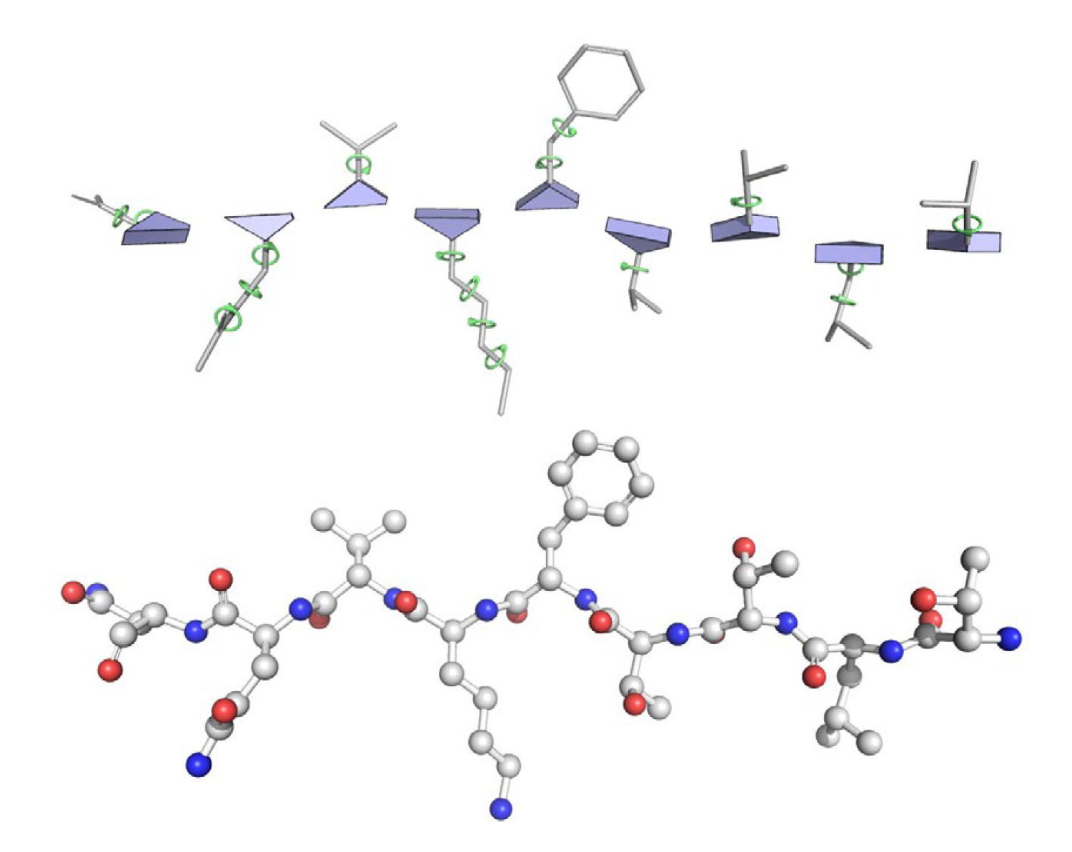
We are now ready to cover what is probably the most complicated yet commonly encountered Riemannian manifold in building machine learning models: the space of rotations in 3D, denoted by $\mathrm{SO}(3)$, the special orthogonal group. Learning rotations is important in frame-based protein structure modeling (see ) and robotics.

Frame construction in AlphaFold2 , where each amino acid is defined by a rotation (frame), a translation (coordinate), and side-chain torsions.

Representing a rotation

Most readers are probably familiar with 3D rotation matrices as an intuitive representation of a rotation: $\begin{equation} \mathrm{SO}(3)=\{R\in\mathbb{R}^{3\times3}:R^\mathsf{T}R=I,\det R=1\}. \end{equation}$ When applied to a 3D vector $x\in\mathbb{R}^3$, the rotation therefore reads as $x\mapsto Rx$. The orthogonality constraint preserves lengths and angles, while the determinant constraint excludes reflections. While rotation matrices offer one possible representation, as $\mathrm{SO}(3)$ is a 3-dimensional manifold, a 3D vector suffices for representing a rotation in principle. The rotation vector representation (axis–angle representation) offers one option. A rotation vector $\theta\in\mathbb{R}^3$ combines an axis and an angle such that the unit vector $\theta/\|\theta\|$ specifies the rotation axis, and $\|\theta\|$ is the angle in radians, following the right-hand rule. For example, $\theta=(0,0,\pi/2)$ rotates the positive $x$-axis onto the positive $y$-axis. The zero vector represents the identity rotation.

Explore a rotation vector

Set the components in units of π.

Drag to orbit · arrow keys also turn the view

φ_x / π

φ_y / π

φ_z / π

Rotation angle 0.5π (90°)

Use numbers or fractions. Each result must be between −1 and 1.

If we choose shortest representatives with $\|\theta\|_2\leq\pi$, we obtain the standard geometric visualization of $\mathrm{SO}(3)$ as a solid 3D ball of radius $\pi$. However, one additional nuance needs to be resolved: the antipodal points on the sphere of this ball (i.e., $\|\theta\|=\pi$) represent the same rotation, since rotating 180 degrees clockwise or counterclockwise gives the same result. We therefore need to additionally identify all the antipodal point pairs on the surface to recover the $\mathrm{SO}(3)$ structure. Such a solid ball representation allows us to intuitively visualize a distribution over rotations and also derive interesting topological properties of $\mathrm{SO}(3)$.

Topological facts about $\mathrm{SO}(3)$

$\mathrm{SO}(3)$ is a non-Abelian group, a property that is probably better known than its manifold structure. Rotations can be composed by matrix multiplication, with identity $I$ and inverse $R^{-1}=R^\mathsf{T}$. Non-Abelian means that the order of applying the rotations matters for the final outcome. Together with its smooth multiplication and inversion, the manifold structure makes $\mathrm{SO}(3)$ a Lie group.
By the rotation vector construction for the solid ball with antipodal identification, $\mathrm{SO}(3)$ is diffeomorphic to the 3D real projective space $\mathbb{RP}^3$.
$\mathrm{SO}(3)$ is path-connected, but not simply connected. This means that $\mathrm{SO}(3)$ and the 3-sphere $S^3$ have different topologies, as the 3-sphere is simply connected. The rotation-vector construction might suggest a connection, but identifying antipodal boundary points changes the topology.
Consider a definition of simple connectedness in which every loop can be shrunk to one point. On the rotation vector solid ball, a loop connecting two antipodal surface points through the interior of the solid ball cannot be shrunk, as the antipodal identification indeed makes it a closed loop.

Poincaré conjecture?

The Poincaré conjecture states that every 3-dimensional closed, simply connected topological manifold is homeomorphic to the 3-sphere. Without simple connectedness, $\mathrm{SO}(3)$ naturally falls outside the scope.

The rotation vector is closely related to the (Lie group) exponential map that connects the tangent vector in the tangent space (Lie algebra) of $\mathrm{SO}(3)$ to a rotation matrix in the Riemannian manifold (Lie group). We will discuss the conversion between them in the following section.

Other common rotation representations

In addition to rotation matrices and rotation vectors, other commonly used representations include:

Unit quaternion. The space of four-dimensional unit quaternions is equivalent to $S^3$, thus forming a double cover (i.e., two-to-one mapping) of $\mathrm{SO}(3)$. Most modern Python packages like SciPy use quaternions as internal storage for rotations, because of their compact representation and convenient slerp support, although most Riemannian generative models still follow AF2’s convention of using rotation matrices and rotation vectors.
Euler angles. A rotation is described by three angles: yaw, pitch, and roll. Euler angles are notorious for their confusing conventions and Gimbal lock, so you should never use them.

Tangent Space of $\mathrm{SO}(3)$

Consider a time-dependent rotation matrix $R(t)$ that satisfies $R(t)^\top R(t)=I$. Differentiating with respect to $t$, we get: $\begin{equation} \dot R^\top R+R^\top\dot R=0. \end{equation}$ Therefore, $\Omega=R^\top\dot R$ is a skew-symmetric matrix that satisfies $\Omega^\top=-\Omega$, and the tangent space at $R$ can be identified as: $\begin{equation} T_R\mathrm{SO}(3)=\{R\Omega:\Omega^\top=-\Omega\}. \end{equation}$

As the base rotation $R$ is known, we only need to learn the skew-symmetric matrix $\Omega$ for generative modeling. The space of all possible $\Omega$ is exactly the tangent space $T_e\mathrm{SO}(3)=\{\Omega:\Omega^\top=-\Omega\}$ at the identity rotation $e=I$. This tangent space of skew-symmetric matrices is known as the Lie algebra $\mathfrak{so}(3)$.

Left Trivialization and Lie Algebra

The representation $V=R\Omega$ above identifies each tangent space $T_R\mathrm{SO}(3)$ with the same vector space $\mathfrak{so}(3)$. This smooth identification is induced by left translation: for $L_{R^{-1}}(Q)=R^{-1}Q$, its differential sends $V$ to $R^{-1}V=\Omega$. Keeping the base point $R$, we obtain a global trivialization of the tangent bundle, with its inverse: $\begin{equation} \begin{aligned} T\mathrm{SO}(3)&\cong\mathrm{SO}(3)\times\mathfrak{so}(3),\\ \Phi(R,V)&=(R,R^{-1}V),\\ \Phi^{-1}(R,\Omega)&=(R,R\Omega). \end{aligned} \end{equation}$

More generally, for any Lie group $G$, let $\mathfrak{g}:=T_eG$. Left translation gives a linear isomorphism $(\mathrm{d}L_g)_e:\mathfrak{g}\to T_gG$ at every $g\in G$, so left-trivialization gives $TG\cong G\times\mathfrak{g}$. Translating a basis of $\mathfrak{g}$ therefore gives smooth vector fields that form a basis at every point, called a global frame. A manifold admitting such a frame is called a parallelizable manifold. This is useful for learning and simulating vector fields. On $\mathrm{SO}(3)$, we can learn a point-dependent and time-dependent skew-symmetric matrix $\Omega_t(R)\in\mathfrak{so}(3)$ and reconstruct the actual tangent velocity as $V_t(R)=R\Omega_t(R)$.

Not every manifold is parallelizable. By the hairy ball theorem, $S^2$ admits no global smooth tangent frame, so we cannot use a single smooth global tangent frame. Local coordinate representations or ambient vectors constrained to the tangent plane still work.

The group structure gives something more specific: every $v\in\mathfrak{g}$ has a unique left-invariant extension $v^L$ to the whole group. These fields are closed under the vector-field Lie bracket, which essentially equips $T_eG$ with its Lie algebra structure.

Explicitly constructing the Lie algebra

For $g,h\in G$, write left translation $L_g(h):=gh$. Its differential is a linear map between tangent spaces: $\begin{equation} (\mathrm{d}L_g)_h:T_hG\to T_{gh}G. \end{equation}$

For a tangent vector $a\in T_hG$ and any smooth function $f:G\to\mathbb{R}$, we have: $\begin{equation} \bigl((\mathrm{d}L_g)_h a\bigr)f=a(f\circ L_g). \end{equation}$

A smooth vector field $V$ is left-invariant if $(\mathrm{d}L_g)_h V_h=V_{gh}$ for all $g,h\in G$. That is, translating the vector gives the same result as evaluating the field at the translated point. Setting $h=e$, we know this vector field is completely determined by $v=V_e\in\mathfrak{g}$.

On the other hand, let $\Gamma(TG)$ denote the space of smooth vector fields and $\Gamma_L(TG)\subseteq\Gamma(TG)$ the left-invariant vector fields. Define the extension map by: $\begin{equation} \begin{aligned} \mathcal{L}:\mathfrak{g}&\longrightarrow\Gamma_L(TG),\\ (v^L)_h&:=(\mathrm{d}L_h)_e(v)\in T_hG. \end{aligned} \end{equation}$

We can verify its left invariance as follows: $\begin{equation} \begin{aligned} (\mathrm{d}L_g)_h(v^L)_h &=(\mathrm{d}L_g)_h(\mathrm{d}L_h)_e(v)\\ &=\mathrm{d}(L_g\circ L_h)_e(v)\\ &=(\mathrm{d}L_{gh})_e(v)=(v^L)_{gh}. \end{aligned} \end{equation}$

Since $(v^L)_e=v$, the map $\mathcal{L}$ is a linear bijection onto $\Gamma_L(TG)$, with inverse given by evaluation at the identity $\mathcal{L}^{-1}(V)=V_e$.

For vector fields, their Lie bracket is defined as: $\begin{equation} [V,W]f:=V(Wf)-W(Vf). \end{equation}$

This is again a smooth vector field, and the bracket is bilinear, antisymmetric, and satisfies the Jacobi identity. We still need to check that $[V,W]$ is left-invariant whenever $V$ and $W$ are. Left invariance gives the function identity $V(f\circ L_g)=(Vf)\circ L_g$, and similarly for $W$. We have: $\begin{equation} \begin{aligned} ((\mathrm{d}L_g)_h[V,W]_h)f &=[V,W]_h(f\circ L_g)\\ &=V_h(W(f\circ L_g))-W_h(V(f\circ L_g))\\ &=V_h((Wf)\circ L_g)-W_h((Vf)\circ L_g)\\ &=V_{gh}(Wf)-W_{gh}(Vf)\\ &=[V,W]_{gh}f. \end{aligned} \end{equation}$

Since this holds for every smooth $f$, we have $(\mathrm{d}L_g)_h[V,W]_h=[V,W]_{gh}$. Thus $\Gamma_L(TG)$ is closed under the bracket. We can now define the Lie bracket on $\mathfrak{g}=T_eG$ by $\begin{equation} [v,w]_{\mathfrak{g}}:=[v^L,w^L]_e. \end{equation}$

Equivalently, $[v,w]_{\mathfrak{g}}^L=[v^L,w^L]$. The bracket on $\mathfrak{g}$ inherits bilinearity, antisymmetry, and the Jacobi identity through $\mathcal{L}$, making $\mathfrak{g}$ a Lie algebra. The construction is summarized below, with the space of each expression underneath: $\begin{equation} \underbrace{(v,w)}_{\mathfrak{g}\times\mathfrak{g}} \xrightarrow{\mathcal{L}\times\mathcal{L}} \underbrace{(v^L,w^L)}_{\Gamma_L(TG)\times \Gamma_L(TG)} \xrightarrow{[\cdot,\cdot]} \underbrace{[v^L,w^L]}_{\Gamma_L(TG)} \xrightarrow{\mathcal{L}^{-1}} \underbrace{[v,w]_{\mathfrak{g}}}_{\mathfrak{g}}. \end{equation}$

The tangent space at the identity is a three-dimensional vector space of skew-symmetric matrices, each with three independent entries: $\begin{equation} \Omega= \begin{pmatrix} 0&-\omega_3&\omega_2\\ \omega_3&0&-\omega_1\\ -\omega_2&\omega_1&0 \end{pmatrix}. \end{equation}$

The hat and vee isomorphisms conveniently convert between a three-dimensional vector $\omega=(\omega_1,\omega_2,\omega_3)$ and its skew-symmetric matrix: $\begin{align} &\hat{(\cdot)}: \mathbb{R}^3\to\mathfrak{so}(3),\quad \omega\mapsto \Omega,\\ &(\cdot)^\vee: \mathfrak{so}(3)\to\mathbb{R}^3,\quad \Omega\mapsto \omega. \end{align}$ Most Riemannian generative models use rotation matrices as the base representation while learning the 3-vector representation defined by the hat-vee isomorphism.

Exponential and Logarithm Maps

Unlike in the preceding manifold sections, we will first cover the exponential and logarithm maps for $\mathrm{SO}(3)$, as the smooth structure of the Lie group already offers a natural way of defining the exponential map without a metric. We will discuss how to choose a “compatible” (bi-invariant) metric in a later section.

Recall the dynamics: $\begin{equation} \dot R=R\Omega. \end{equation}$ For constant $\Omega$, solving the ODE with $\gamma(0)=R$ and $\dot\gamma(0)=R\Omega$ gives the curve below. It is a Riemannian geodesic for the bi-invariant metric introduced later: $\begin{equation} \gamma(t)=R\operatorname{Exp}(t\Omega), \end{equation}$ where $\operatorname{Exp}$ denotes matrix exponentiation that can be defined using the power series: $\begin{equation} \operatorname{Exp}(X) = \sum_{k=0}^{\infty} \frac{X^{k}}{k!} = I + X + \frac{1}{2}X^{2} + \frac{1}{6}X^{3} + \cdots \end{equation}$

Setting $t=1$ and using the 3-vector representation with the hat isomorphism gives the exponential map. Here, $\omega$ denotes left-trivialized coordinates: the actual tangent vector at $R$ is $R\hat\omega$. $\begin{equation} \boxed{\exp_R(\omega)=R\operatorname{Exp}(\hat \omega), \quad \omega\in \mathbb{R}^3}.\label{eqn:riemann_exp} \end{equation}$ Similarly, using the matrix logarithm represented near the identity by the convergent power series (for $\|I-B\|_2<1$) $\begin{equation} \operatorname{Log}(B) = -\sum_{k=1}^{\infty} \frac{(I-B)^{k}}{k} = -(I-B) - \frac{(I-B)^{2}}{2} - \frac{(I-B)^{3}}{3} - \cdots, \end{equation}$ we can obtain the formal solution of the logarithm map using the three-vector representation and the vee isomorphism: $\begin{equation} \boxed{\log_{R_1}(R_2)=(\operatorname{Log}(R_1^\top R_2))^\vee \in \mathbb{R}^3}.\label{eqn:riemann_log} \end{equation}$

In the derivation above, we rely only on algebraic results to obtain an important corollary: the matrix exponential $\operatorname{Exp}:\mathfrak{so}(3)\to\mathrm{SO}(3)$ sends a skew-symmetric matrix to a rotation matrix, while choosing a real skew-symmetric logarithm maps a rotation matrix back to $\mathfrak{so}(3)$. We use the shortest branch; it is unique for rotation angles below $\pi$.

Direct verification of the $\mathrm{SO}(3)$ vs $\mathfrak{so}(3)$ connection

Matrix exponential. Let $R=\operatorname{Exp} \Omega$ for a skew-symmetric matrix $\Omega\in\mathfrak{so}(3)$. Notice that $(\operatorname{Exp} \Omega)^\top=\operatorname{Exp}(\Omega^\top)=\operatorname{Exp}(-\Omega)$. Since $-\Omega$ and $\Omega$ commute, we have: $\begin{equation} R^\top R=\operatorname{Exp}(-\Omega)\operatorname{Exp}(\Omega)=\operatorname{Exp}(0)=I. \end{equation}$ Additionally, $\operatorname{Exp}(\Omega)=\operatorname{Exp}(\Omega/2)\operatorname{Exp}(\Omega/2)$ gives $\det R=(\det \operatorname{Exp}(\Omega/2))^2>0$. Together with orthogonality, this shows that $R$ is a rotation matrix.

Matrix logarithm. For this local series proof, take $R$ sufficiently close to $I$, for example $\|R-I\|_2<1/2$, and let $\Omega=\operatorname{Log} R$. Note that $\Omega^\top = \operatorname{Log} R^\top=\operatorname{Log}R^{-1}$. We have: $\begin{equation} \begin{aligned} \operatorname{Log}R^{-1}&=-\sum_{k=1}^{\infty}\frac{(R-I)^k}{k}(I+(R-I))^{-k}\\ &=-\sum_{k=1}^{\infty}\frac{(R-I)^k}{k}\sum_{j=0}^\infty(-1)^j\binom{k+j-1}{j}(R-I)^j\\ &=-\sum_{n=1}^{\infty}\sum_{k=1}^{n}\frac{(-1)^{n-k}}{k}\binom{n-1}{k-1}(R-I)^n\\ &=-\sum_{n=1}^{\infty}\sum_{k=1}^{n}\frac{(-1)^{n-k}}{n}\binom{n}{k}(R-I)^n\\ &=-\sum_{n=1}^{\infty}\frac{1}{n}[(1-1)^n-(-1)^n](R-I)^n\\ &=-\sum_{n=1}^{\infty}\frac{(-1)^{n+1}}{n}(R-I)^n=-\operatorname{Log}R, \end{aligned} \end{equation}$ where in the third equation we collect terms with $n=k+j$. Therefore, $\Omega^\top=-\Omega$, so $\Omega$ is skew-symmetric.

The exponential series converges for every matrix. The logarithm series is local; the bound above also justifies the double-series rearrangement. Choosing a principal logarithm does not extend the convergence region of this series. For larger rotations, we use the closed-form expressions below.

Every Lie group admits a Lie group exponential map $\operatorname{Exp}:\mathfrak{g}\to G$ and a local logarithm near the identity. For matrix Lie groups, these agree with the matrix exponential and its local inverse.

Direct calculation of matrix exponentials and logarithms is expensive. Luckily, they have closed-form expressions for $\mathrm{SO}(3)$. The key is to notice the recurring pattern of the unit skew-symmetric matrix: $K^3=-K,\|K^\vee\|_2=1$. This can be directly verified numerically or by calculating the characteristic polynomial $\det (K-tI)=-t^3-t$ with the Cayley–Hamilton theorem. In this way, writing $K=\hat\omega/\|\omega\|$, we can collect all terms in the exponential power series into finitely many matrix terms: $\begin{equation} \begin{aligned} R&=\operatorname{Exp}(\|\omega\| K)=\sum_{k=0}^\infty\frac{(\|\omega\| K)^k}{k!}\\ &=I + \left(\|\omega\| - \frac{\|\omega\|^3}{3!} + \frac{\|\omega\|^5}{5!} - \cdots\right) K \\ &\quad+ \left(\frac{\|\omega\|^2}{2!} - \frac{\|\omega\|^4}{4!} + \frac{\|\omega\|^6}{6!} - \cdots\right) K^2\\ &= I +K \sin\|\omega\| + (1-\cos\|\omega\|) K^2. \end{aligned} \end{equation}$ Substituting $K=\hat\omega/\|\omega\|$ back, we obtain Rodrigues’ rotation formula (with its continuous limit at $\omega=0$): $\begin{equation} \boxed{R=\operatorname{Exp}(\hat\omega)=I+\frac{\sin\|\omega\|}{\|\omega\|}\hat\omega+\frac{1-\cos\|\omega\|}{\|\omega\|^2}\hat\omega^2}.\label{eqn:lie_exp} \end{equation}$

For the logarithm, we first note that the only anti-symmetric part in Rodrigues’ formula is the $\hat\omega$ component. Therefore, we have $R-R^\top=2\hat\omega\sin\|\omega\|/\|\omega\|$. Additionally, note that $\operatorname{tr}(\hat\omega^2)=-2(\omega_1^2+\omega_2^2+\omega_3^2)=-2\|\omega\|^2$. Taking the trace on both sides, we have: $\begin{equation} \operatorname{tr} R=3-2(1-\cos\|\omega\|)=1+2\cos\|\omega\|.\label{eqn:rot_trace} \end{equation}$

Combining these two results, for $0<\|\omega\|<\pi$, the shortest logarithm is: $\begin{equation} \boxed{\hat\omega=\operatorname{Log}(R)=\frac{\|\omega\|}{2\sin\|\omega\|}(R-R^\top),\quad \|\omega\|=\arccos \frac{\operatorname{tr} R-1}{2}}.\label{eqn:lie_log} \end{equation}$

Geometric Rederivation of Both Maps

So far, we have derived both the Lie group exponential map in Eq. \eqref{eqn:lie_exp} and logarithm map in Eq. \eqref{eqn:lie_log} (thus the Riemannian maps in Eq. \eqref{eqn:riemann_exp} and \eqref{eqn:riemann_log}) using purely algebraic derivations, without any geometric intuition. We now offer an alternative perspective to rederive the exponential and logarithm maps from a purely geometric perspective.

Intuitively, as $\mathrm{SO}(3)$ is transitive on itself, which means we can connect any two rotations with another rotation, the relative rotation $R_1^\top R_2$ determines the left-trivialized tangent vector through its Lie logarithm, as in Eq. \eqref{eqn:riemann_log}. Additionally, to construct a geodesic with a constant velocity that aligns one rotation to another, the most intuitive way is to find a fixed rotation axis with a constant angular velocity. This naturally aligns with the rotation vector representation.

Indeed, from the above algebraic derivation, we can confirm this mathematically. Recall that the trace is invariant under change of basis. Now consider a shortest rotation vector aligned with the $z$-axis. Its rotation matrix in that frame then takes the canonical form of $\operatorname{diag}\{(\begin{smallmatrix}\cos\theta&-\sin\theta\\ \sin\theta&\cos\theta\end{smallmatrix}),1\}$, with $\theta\in[0,\pi]$ being the rotation angle. Therefore, the trace of a rotation matrix is exactly $1+2\cos\theta$. Comparing with Eq. \eqref{eqn:rot_trace}, we immediately obtain the geometric interpretation: $\begin{equation} \|\omega\|=\theta. \end{equation}$ That is, the left-trivialized tangent vector of the connecting geodesic is the relative rotation vector. With this connection, we can treat $\omega$ as a rotation vector and also rederive the exponential map purely geometrically.

Geometric construction of the exponential and logarithm maps

To keep the geometric intuition simple, we consider $0<\theta=\|\omega\|<\pi$ and nonzero perpendicular components. For the logarithm, we assume the selected rows are independent; the identity and half-turn cases are omitted.

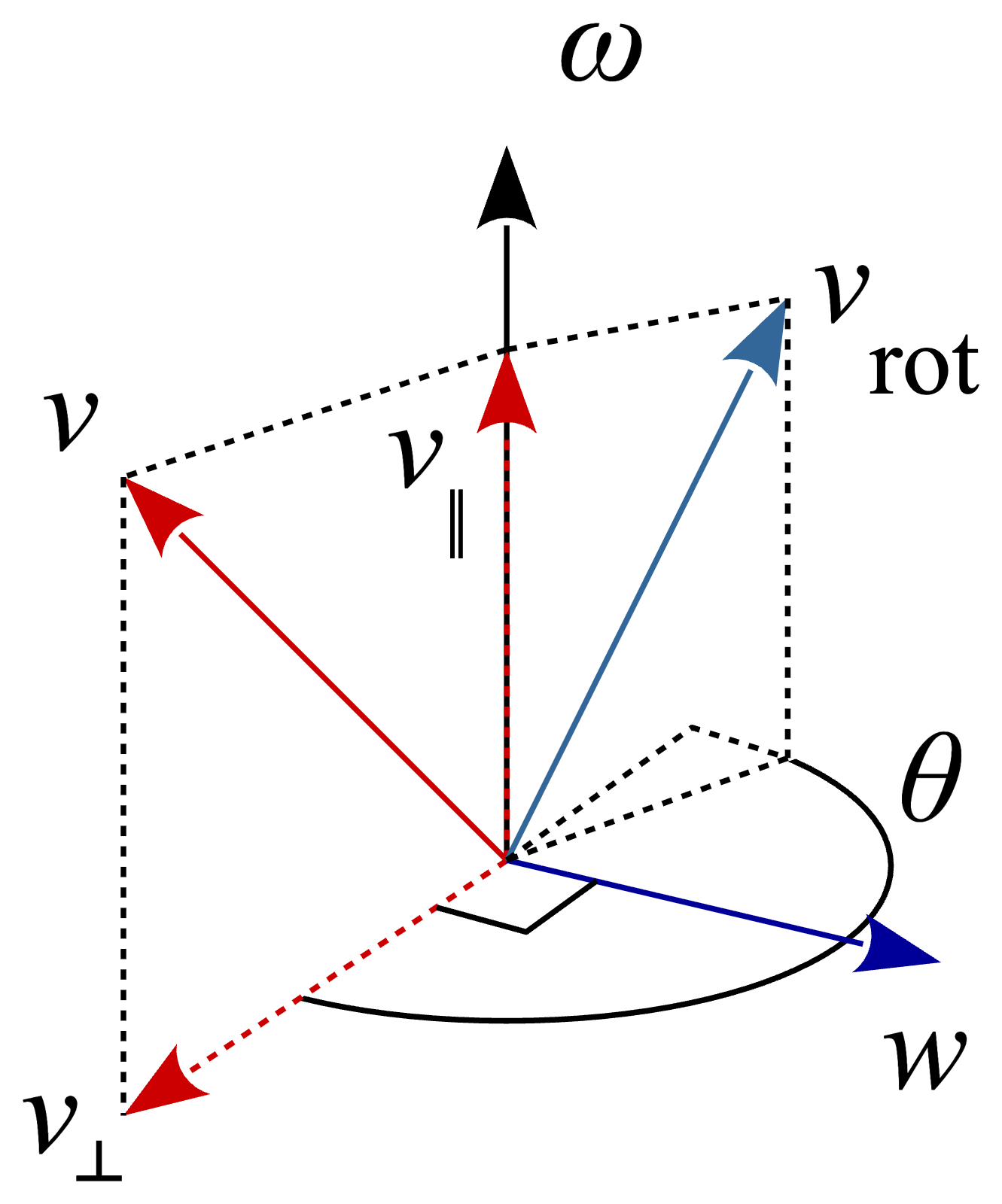
Exponential map. Consider a three-dimensional vector $v\in\mathbb{R}^3$. We want to obtain the rotated vector $v_\text{rot}$ about the axis $\omega$ with a rotation angle $\theta=\|\omega\|$. After decomposing $v$ into parallel and orthogonal components (see ), it is easy to see that the parallel component $v_{\|}$ remains unchanged while the orthogonal component $v_\perp$ rotates by $\theta=\|\omega\|$ as we discussed for the spherical manifold. In this way, we have: $\begin{equation} v_\text{rot}=v_{\|}+v_\perp\cos\theta+w\sin\theta, \end{equation}$ where $w$ is perpendicular to both $\omega$ and $v$, follows the right-hand rule, and has length $\|v_\perp\|$, as in the figure.

Let $k=\omega/\|\omega\|$ denote the unit rotation-axis direction. We can calculate the decomposition of $v$ as: $\begin{equation} v_{\|}=\langle v,k\rangle k,\quad v_\perp=v-v_{\|}=-k\times(k\times v), \end{equation}$ where $\times$ is the cross product. Also note that $\|k\times v\|=\|v_\perp\|$, so $w=k\times v$. Therefore, $\begin{equation} \begin{aligned} v_\text{rot}&=v-(1-\cos\theta)v_\perp+(k\times v)\sin\theta\\ &=v+k\times v\sin\theta+(1-\cos\theta)k\times(k\times v). \end{aligned} \end{equation}$ Substituting $k=\omega/\|\omega\|$ back, we have: $\begin{equation} v_\text{rot}=v+\frac{\sin\|\omega\|}{\|\omega\|}\omega\times v+\frac{1-\cos\|\omega\|}{\|\omega\|^2}\omega\times(\omega\times v), \end{equation}$ which is also called Rodrigues’ rotation formula and is consistent with Eq. \eqref{eqn:lie_exp}.

Rodrigues' rotation geometry with axis omega, original vector v, its parallel and perpendicular components, and the rotated vector. — Geometric construction of Rodrigues' rotation formula.

Logarithm map. An axis direction $p$ that rotates a unit vector $u$ into another unit vector $v$ must satisfy $p\cdot(u-v)=0$, since rotation preserves the component along the axis. Let $x,y,z$ denote the coordinate unit vectors. A rotation matrix $R=(u,v,w)$ sends them to its three columns, so its axis satisfies: $\begin{equation} (R^\top-I) p=0. \end{equation}$ Note that $\begin{equation} \begin{aligned} \det (R^\top-I)&=\det (R-I)=\det R\det (I-R^\top)\\ &=\det (I-R^\top) = (-1)^3\det (R^\top-I)\\ &=-\det (R^\top-I), \end{aligned} \end{equation}$

so $\det(R^\top-I)=0$. Assuming the first two rows are independent, an axis direction is $p=(u-x)\times(v-y)$. Since $R-R^\top=-(R+I)(R^\top-I)$, we also have $(R-R^\top)p=0$. For $0<\theta<\pi$, this means $p$ is parallel to the axis vector $(R-R^\top)^\vee$. Any other independent pair of rows gives the same axis, up to scale and sign. Choose the sign so that $p\cdot(R-R^\top)^\vee>0$.

The rotation angle is the angle between the projections of $u$ and $x$ onto the plane perpendicular to $p$. Let $k=p/\|p\|$; then $u\cdot k=x\cdot k$. Using the law of cosines on the distance between $u$ and $x$, we have: $\begin{equation} 2(1-u\cdot x)=2(1-(k\cdot x)^2)(1-\cos\theta). \end{equation}$

So $(1-\cos\theta)(1-k_1^2)=(1-u_1)$. Using the other two axes similarly yields $(1-\cos\theta)(1-k_2^2)=(1-v_2)$ and $(1-\cos\theta)(1-k_3^2)=(1-w_3)$. Adding the three equations together with $k_1^2+k_2^2+k_3^2=1$, we get: $\begin{equation} 2(1-\cos\theta)=3-u_1-v_2-w_3=3-\operatorname{tr}(R), \end{equation}$ This recovers $2\cos\theta=\operatorname{tr}(R)-1$ and hence the rotation vector $\omega=\theta p/\|p\|$.

Metric for $\mathrm{SO}(3)$

Both the algebraic and geometric derivations of the exponential and logarithm maps already offer a solid and intuitive way of defining the geodesic distance and the corresponding metric.

With the connection between the shortest rotation vector $\omega$ and the relative rotation matrix, we naturally define its rotation angle as the geodesic distance: $\begin{equation} d_{\mathrm{SO}(3)}(R_1,R_2)=\|\operatorname{Log}(R_1^\top R_2)^\vee\|_2, \end{equation}$ where $R_1^\top R_2$ is the relative rotation. This definition also exhibits one desirable property: the distance depends only on the relative rotation and is invariant to global rotations $R\in \mathrm{SO}(3)$: $\begin{equation} d_{\mathrm{SO}(3)}(R R_1,R R_2)=d_{\mathrm{SO}(3)}(R_1 R, R_2 R)=d_{\mathrm{SO}(3)}(R_1,R_2). \end{equation}$ We call this distance bi-invariant as it is both left-invariant and right-invariant with respect to group actions. This distance induces a bi-invariant metric. For $V_1=R\Omega_1, V_2=R\Omega_2\in T_R\mathrm{SO}(3)$, we have $\begin{equation} g_R(V_1,V_2)=\frac12\operatorname{tr}(V_1^\top V_2)=\frac12\operatorname{tr}(\Omega_1^\top \Omega_2). \end{equation}$ That is, the metric is independent of the point $R$ when the left-trivialized representation $\Omega$ is used. Using the hat-vee isomorphism, the metric reduces to: $\begin{equation} g_R(\omega_1,\omega_2)=\langle\omega_1, \omega_2\rangle,\quad \|\omega\|_{\mathrm{SO}(3)}=\|\omega\|_2, \end{equation}$ The $1/2$ coefficient ensures that the tangent norm agrees with the Euclidean norm of the rotation vector.

Why does bi-invariance matter?

While we may hope that every Lie group admits a bi-invariant metric, it turns out that it does not always exist. $\mathrm{SE}(3)$ is a famous example, where both left-invariant and right-invariant Riemannian metrics exist, but no bi-invariant Riemannian metric exists. So intuitively speaking, a bi-invariant metric ensures that the Lie geodesic (defined by the left-invariant vector field) is the same as the Riemannian geodesic for that metric. For $\mathrm{SE}(3)$, Riemannian geodesics generally have nonconstant left-trivialized velocity.

Nonetheless, for Riemannian generative modeling, both paths are valid as long as the vector field is correctly calculated and regressed. It is like choosing variance-preserving paths or optimal-transport paths for flow matching on Euclidean space: the choice of probability path on a Lie group is a design decision. For a Lie group with a bi-invariant metric, these two coincide, offering a more “canonical” way of defining the geometry.

The numerical stability issues are more pronounced with $\mathrm{SO}(3)$ in practical machine learning implementations. An example of a numerically stable implementation can be found in my codebase.