A Less Mathematical Introduction to Tensor Field Networks
Introduction
Equivariance has been a long-standing concern in various fields including computer vision
I will skip any mathematical proof and focus on the intuition behind the model. Nonetheless, some mathematical definitions of equivariance will be provided and some mathematical background is still required to understand the model. I will assume the reader has basic knowledge of linear algebra and group theory. So, let’s get started!
Equivariance
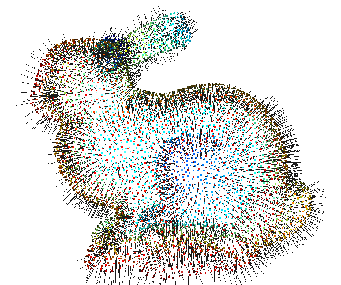
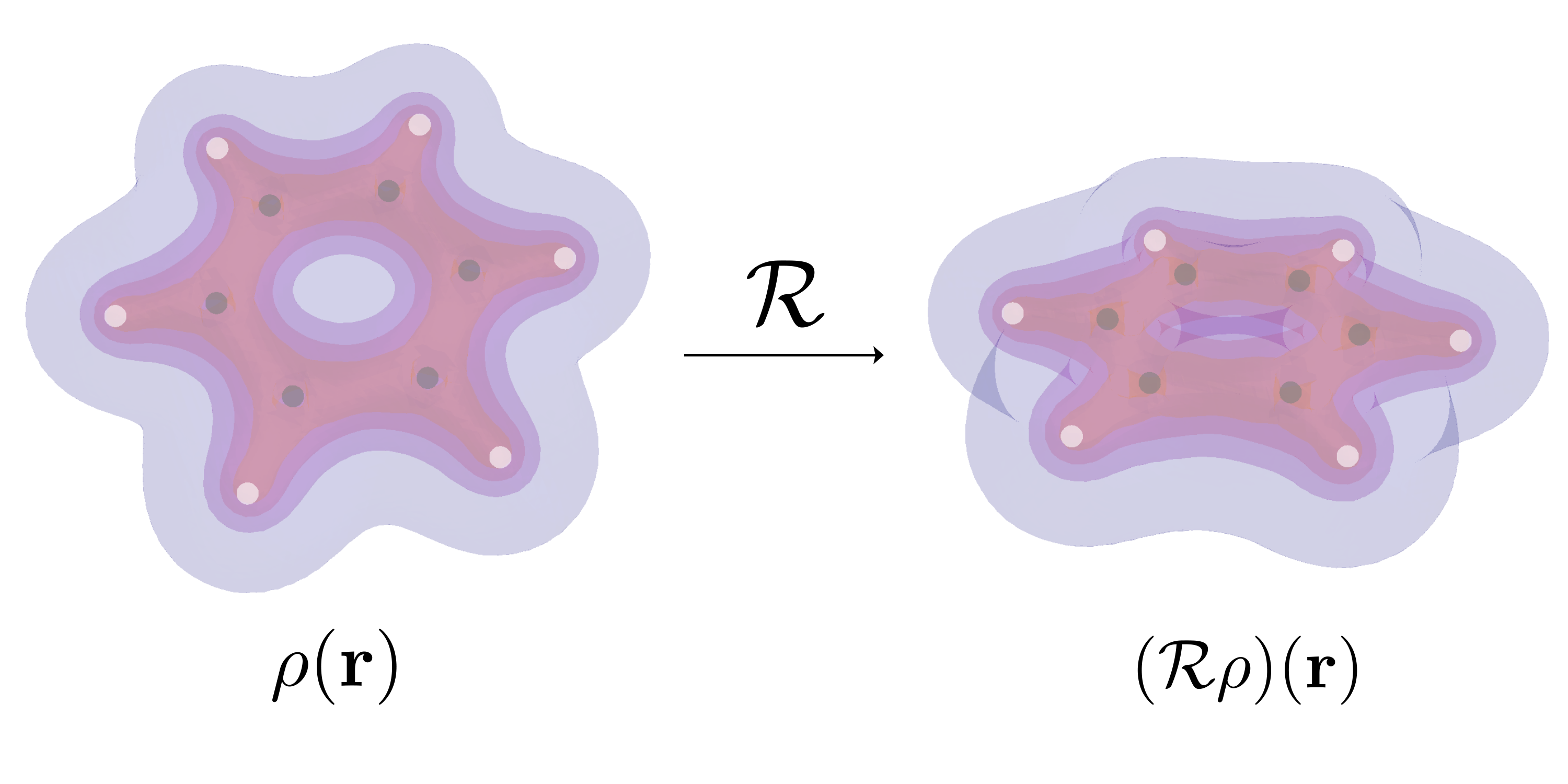
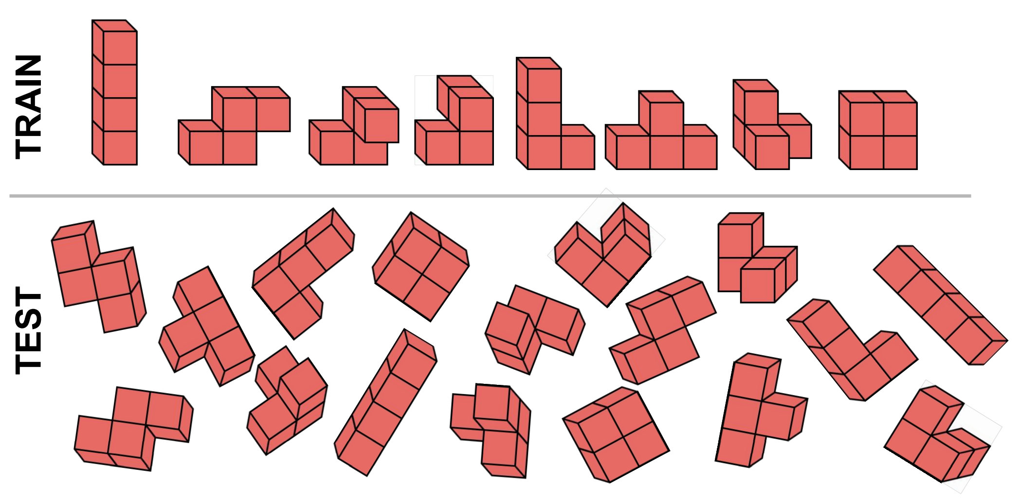
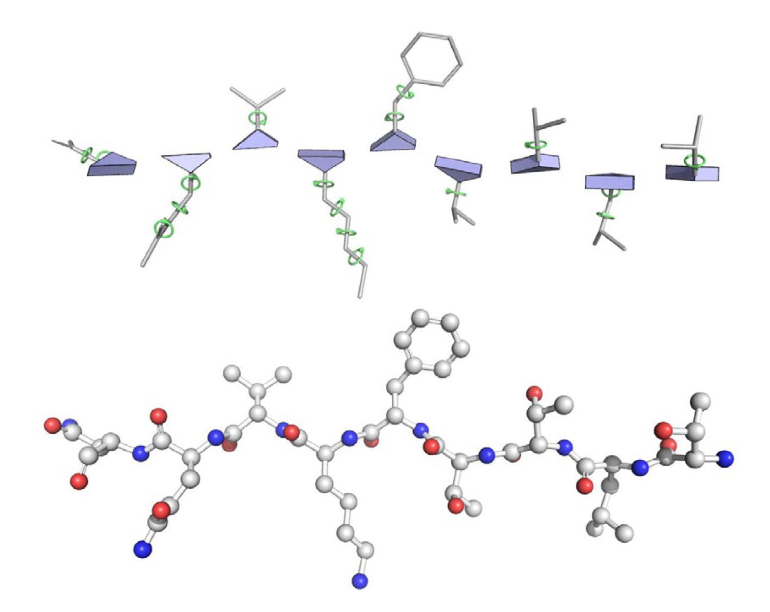
In 3D Euclidean space, many properties are independent of the poses of the object. Some examples are shown in . For normal estimation on 3D point clouds, the normal vector will rotate with the global rotation. The electron density mapping will also rotate accordingly with the rotation of the atom coordinates. An ideal model in such scenarios should be robust to the transformation such that it makes predictions that also transform accordingly. In other words, the model is equivariant to the global transformation. The last example demonstrates the invariance property on the classification task, as we would naturally expect the classifier to output consistent results no matter how we rotate the Tetris block.
Therefore, equivariance demonstrates the robustness of the model in a way that it is independent of the global rotation of the input. It also serves as an implicit way of data augmentation, as the model can be thought of as being trained on the whole trajectory of every data point.
Mathematically, we can intuitively define the equivariance property of some function $f$ such that for any transformation $g$, it is equivalent to apply $g$ inside $f$ as to apply $g$ outside $f$, or in other words, $f(gx)=gf(x)$. We will use a slightly generalized definition of equivariance as follows:
One benefit of such a definition of equivariance is that we can easily extend it to invariance by setting $\mathcal{T}:g\mapsto e$: \begin{equation} f(g\cdot x)=f(x),\forall g\in G,x\in X \label{eqn:inv} \end{equation}
In this way, invariance can be viewed as a special case of equivariance. I will show how this generalization is important when we try to extend the concept of equivariance to spherical tensors with Wigner D-matrices.
As the 3D Euclidean space is commonly encountered in real-world data and tasks, we will focus on the 3D special Euclidean group SE(3) which consists of all rigid isometries. In most cases, the translation equivariance can be obtained by using the relative coordinates $\mathbf{r}_{uv}=\mathbf{x}_v-\mathbf{x}_u$. Therefore, rotation equivariance is of more importance, and we will mainly consider the special orthogonal group SO(3) which consists of all rotation matrices.
Previous Works
It is beneficial to review other model architectures designed to achieve equivariance and/or invariance before TFN. Here, the common definitions of equivariance and invariance suffice, i.e., $f(R\mathbf{x})=Rf(\mathbf{x})$ for equivariance and $f(R\mathbf{x})=f(\mathbf{x})$ for invariance. Roughly they can be categorized into three groups: 1) invariant nets, 2) local frame-based nets, and 3) vector neuron-based nets.
The invariant nets are probably the most intuitive architecture by using only the invariant features as input. As any global rotation will not change the feature, the model will still receive the same input features after rotation, trivially achieving equivariance. Invariant features include scalars like distance, angle, and dihedral angle; node and edge attributes such as categorical node types and edge types; and also any functions of these invariant features. These models include many classic GNNs like SchNet
Local frame-based nets leverage the fact that, when a local canonical frame can be assigned, equivariance can be achieved by transforming the input features into the local canonical frame. One noticeable example is AlphaFold2 by DeepMind
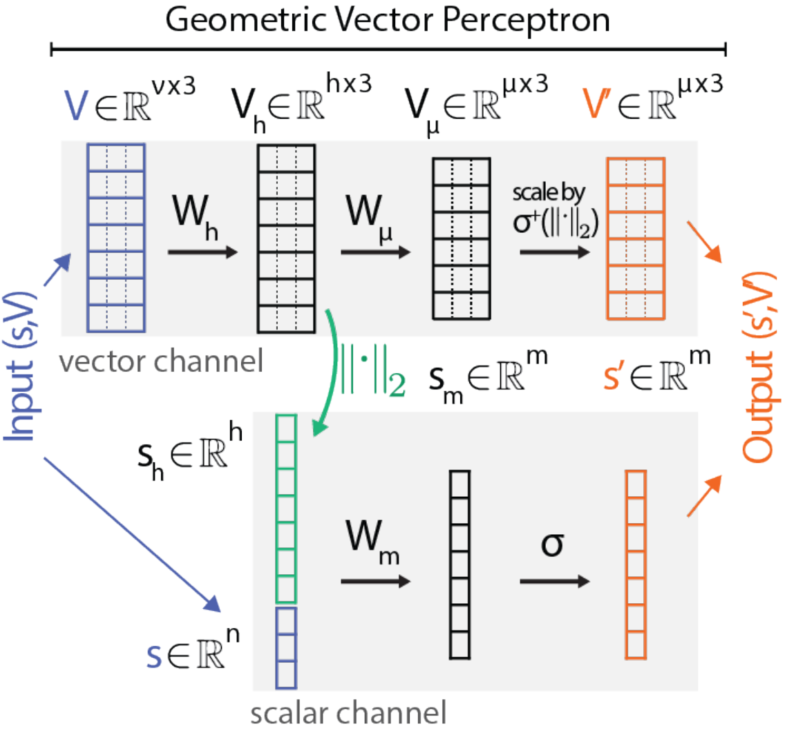
Vector neuron-based nets
Tensor Field Network
Before formally introducing the TFN architecture, we shall first review some ways of making new equivariant functions. Suppose $f,g:\mathbb{R}^3\to \mathbb{R}^3$ are equivariant functions satisfying Eq.\eqref{eqn:eqv}, then it can be easily shown that their linear combination $af+bg$ and composition $g\circ f$ are also equivariant. Tensor product provides a third alternative: $f\otimes g$ is also equivariant and transforms according to the following equation: \begin{equation} \mathcal{D} f \otimes \mathcal{D}^{\prime} g=\left(\mathcal{D} \otimes \mathcal{D}^{\prime}\right)(f \otimes g) \end{equation} where $\mathcal{D},\mathcal{D}^{\prime}$ are Wigner D-matrices and $\mathcal{D} \otimes \mathcal{D}^{\prime}$ is the Kronecker product of them
Wigner D-Matrix
Recall that when defining equivariance, we generalize the condition so that every rotation can be moved outside the function up to a group homomorphism. The irreducible representation of SO(3) provides such a homomorphism by mapping each group element $\mathcal{R}$ (a rotation) into a Wigner D-matrix $\mathcal{D}^\ell_\mathcal{R},\ell\ge 0$. Each Wigner D-matrix $\mathcal{D}^\ell$ of degree $\ell$ is a $(2\ell+1)\times (2\ell+1)$ unitary matrix. By leveraging this homomorphism, if we define a spherical tensor to be a collection of $(2\ell+1)$-dimensional vectors, $\mathsf{a}=\{\mathbf{a}^\ell,\ell\ge 0\}$
We can write it in a more compact form: \(\mathcal{R}\mathsf{a}=\mathcal{D}_\mathcal{R}\mathsf{a}\). Let’s check a few examples. When \(\ell=0\), we have \(\mathcal{D}^0_\mathcal{R}=1\) which indicates that scalars are invariant under rotation. When \(\ell=1\), we have \(\mathcal{D}^1_\mathcal{R}=R\) where $R$ is the rotation matrix associated with the rotation $\mathcal{R}$. This is also consistent with the normal definition of rotation. Then, the equivariance condition can be written as:
It is possible to further define the equivariance condition for a matrix, but it turns out that it is unnecessary, as there exists a way to reduce the tensor product of two spherical tensors to another spherical tensor. By this reduction, we can also avoid the problem that the dimensionality of the tensor product will grow exponentially.
Reducing Tensor Product
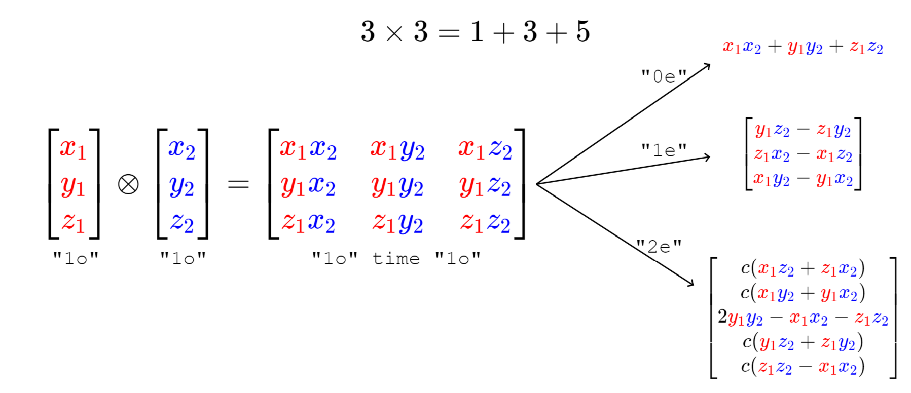
demonstrates the example of reducing the tensor product of two 3D vectors. By rearranging and linearly combining the terms in the 3-by-3 matrix, we can produce a scalar, a 3D vector, and a 5D vector that transform according to the Wigner D-matrices of degree 0, 1, and 2, respectively. It is easy to see the scalar here is the inner product of two vectors, which is invariant; and the 3D vector is the vector product of them, which is equivariant. Generally, the tensor product of an $L_1$-dimensional vector and an $L_2$-dimensional vector can be reduced as \begin{equation} L_{1} \otimes L_{2}=\left|L_{1}-L_{2}\right| \oplus \cdots \oplus\left(L_{1}+L_{2}\right) \end{equation}
One way of defining the tensor product for two spherical tensors arises from the coupling of angular momentum in quantum mechanics. The tensor product $\mathsf{c}=\mathsf{a}\otimes \mathsf{b}$ is defined as \begin{equation} C_{J m}=\sum_{m_{1}=-\ell}^{\ell} \sum_{m_{2}=-k}^{k} a_{\ell m_{1}} b_{k m_{2}}\langle\ell m_1 k m_2 | Jm\rangle \label{eqn:tp} \end{equation} where the 6-index coefficients $\langle\ell m_1 k m_2 | Jm\rangle$ are known as the Clebsch-Gordan coefficients. The Clebsch-Gordan coefficients are nonzero when $|\ell-k|\le J\le \ell+k,-J\le m\le J$, and the reduction of the tensor product can be done by the summation over the indices $J m$.
Equivariant Message Passing
Leveraging the equivariance property of the tensor product, we can define an equivariant message passing scheme as: \(\begin{equation} \mathsf{x}_{u} \leftarrow \sum_{v \in \mathcal{N}_{u}} \sum_{\ell k} w_{\ell k} \sum_{J m} \mathsf{r}_{u v} \otimes \mathsf{x}_{v} \label{eqn:mp} \end{equation}\) where \(\{\mathsf{x}_u\}_{u\in \mathcal{V}}\) are node-wise spherical tensor features, \(\{\mathsf{r}_{uv}\}_{uv\in \mathcal{E}}\) are edge-wise spherical tensor features capturing the geometric information, and $w_{\ell k}$ are learnable weights. Note that the tensor product of two spherical tensors gives a four-dimensional tensor indexed by $\ell,k,J,m$. The innermost summation over $Jm$ is the reduction of the tensor product. The outermost summation is the message-passing paradigm that aggregates information from the neighboring nodes. The middle summation with the learnable weights parameterizes the tensor product from the degree $k$ component of the neighboring node to the degree $\ell$ component of the center node.
The message passing scheme in Eq.\eqref{eqn:mp} is equivariant as it is a linear combination of equivariant tensor products. The rest of the problem is, how can we generate equivariant spherical tensor features? It is convenient to find scalar and (3D) vector features. But for higher-degree features, it is non-trivial to generate them. Luckily, the spherical harmonics provide a solution.
Spherical Harmonics
The spherical harmonics $Y^m_\ell(\hat{\mathbf{r}}),\ell\ge 0,-\ell\le m\le\ell$ are defined on the surface of the unit sphere $S^2$. The degree $\ell$ spherical harmonics has exactly $2\ell+1$ components that together form an equivariant polynomial $Y_\ell:\mathbb{R}^3\to\mathbb{R}^{2\ell+1}$ such that \begin{equation} Y_\ell (R\hat{\mathbf{r}})=\mathcal{D}^\ell_\mathcal{R}Y_\ell (\hat{\mathbf{r}})\label{eqn:sh} \end{equation}
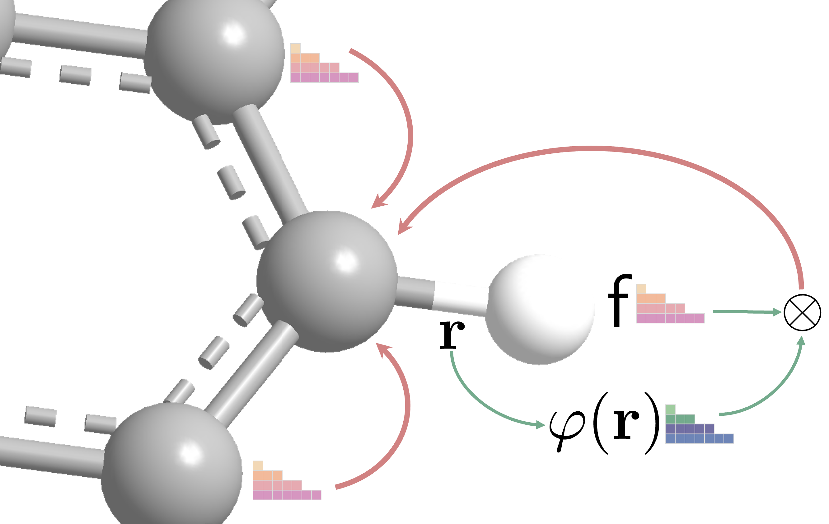
The spherical harmonics are also closely related to the SO(3) group as they are the orthonormal basis functions for irreducible representations of SO(3). But for now, we will only focus on their equivariance property. As the spherical harmonics only capture the direction information of $\hat{\mathbf{r}}$, we need to inject information of the edge distance $r=|\mathbf{r}|$. In TFN, the edge-wise tensor features are defined as \(\begin{equation} \mathsf{r}=\{\varphi_\ell(r) Y_\ell^m(\hat{\mathbf{r}}),\ell\ge 0,-\ell\le m\le \ell\} \label{eqn:edge} \end{equation}\) where $\varphi_\ell(r):\mathbb{R}\to\mathbb{R}$ is a learnable radial network capturing the distance information. Note that the learnable radial network is independent of the spherical harmonics order $m$ such that the angular part of the spherical tensor is completely constrained. It can be shown that as the rotation of the spherical harmonics transforms into a linear combination of the spherical harmonics of the same degree (Eq.\eqref{eqn:sh}), the edge tensor features defined above are equivariant. On the other hand, if the radial net can depend on the order $m$, the equivariance property is no longer preserved.
For node-wise tensor features, it can be shown by induction that if the initial node tensors are equivariant, then the output tensor will also be equivariant after an arbitrary number of message-passing layers. In practice, TFN just used the scalar features and 3D vector features as the initial node-wise tensor features ($\ell\le 1$). The hidden tensor features can have larger degrees, as the tensor product of a degree $\ell$ vector and a degree $k$ vector will give a nonzero coefficient of a degree $\ell+k$ vector.
Putting Everything Together
We finally arrive at the time to put everything together! Plugging the numerical expression of tensor product in Eq.\eqref{eqn:tp} and the edge tensor features in Eq.\eqref{eqn:edge} into the equivariant message passing scheme in Eq.\eqref{eqn:mp}, we get the vectorized form of the message passing scheme in TFN: \(\begin{equation} \mathbf{x}_u^\ell=\sum_{v\in\mathcal{N}(u)}\sum_{k\ge 0}\sum_{J=|k-\ell|}^{k+\ell}\hat{\varphi}_J^{\ell k}(r)\sum_{m=-J}^{J}Y^m_J(\hat{\mathbf{r}})Q_{Jm}^{\ell k}\mathbf{x}^k_v \label{eqn:tfn} \end{equation}\) where $Q_{Jm}^{\ell k}(m_1 m_2)=\langle \ell m_1 k m_2|Jm\rangle$ is the Clebsch-Gordan matrices, and \(\hat{\varphi}_J^{\ell k}(r)=w_{\ell k}\varphi_J(r)\). Here, we coalesce the learnable weights into the learnable radial functions so that all the learnable parts are \(\hat{\varphi}_J^{\ell k}(r)\)
Now, let us consider stacking multiple message-passing layers. We shall consider the nonlinear activation function between layers. Unfortunately, most elementwise activations like ReLU are not generally equivariant. For example, consider a 3D vector in the first octant, the ReLU activation will map any rotated components outside the first octant to zero but preserve other components. Inspired by this finding, we shall consider every degree $\ell$ component of the spherical tensor as a whole and apply the activation function component-wise. TFN uses the 2-norm of each component in the nonlinearity: \(\begin{equation} \mathbf{x}^\ell\gets \sigma^\ell\left(\|\mathbf{x}^\ell\|_2+b^\ell\right) \mathbf{x}^\ell \end{equation}\) where $b^\ell$ is some learnable bias and $\sigma^\ell$ is some differential activation function. Note that $\mathcal{D}^\ell$ is unitary, so for any $\mathcal{R}$, we have \(\|\mathcal{D}^\ell_\mathcal{R}\mathbf{x}^\ell\|_2 =\|\mathbf{x}^\ell\|_2\) which guarantees the equivariance.
Discussion
As we have seen, TFN has a strong theoretical guarantee that the model will be equivariant by design, and it is also free of any pre-assigned local frames. As for the cost, the TFN architecture is quite complicated and hard to implement with high time complexity. Specifically,
- The time complexity of a message passing layer is of order $O(|\mathcal{E}|C(\ell+1)^6)$ where \(C\) is the number of channels. This is because the message passing step involves a tensor product of two spherical tensors and the Clebsch-Gordan coefficients have their six indices all summed. The sextic dependence on $\ell$ makes it prohibitive to use a large $\ell$ in practice.
- The spherical tensor is jagged, as it contains vectors of different dimensionality. This makes it hard to implement the tensor product efficiently. Either a mask needs to be applied to the tensor product, or it needs to be implemented in a sparse manner. The former is not efficient, and the latter is not easy to implement.
- The spherical harmonics need to be computed on the fly, as they take the edge direction $\hat{\mathbf{r}}$ as input. To make things even worse, the spherical harmonics contain associated Legendre polynomials which need to be evaluated recursively. The Clebsch-Gordan coefficients, on the other hand, though also complicated, can be precomputed once and stored for the whole training and evaluation.
For the first problem, current learning scenarios have almost all input features and target features of degree 0 or 1. For the latter two problems, there exists off-the-shelf Python libraries, most noticeably, e3nn which is built upon PyTorch. We can build a parameterized tensor product with e3nn’s high-level interfaces which wrap all the intricate index manipulation and summation with the Clebsch-Gordan coefficients. In e3nn’s implementation, the spherical tensor is stored in a dense vector. For example, a spherical tensor with a degree up to $\ell$ has $(\ell+1)^2$ elements that can be stored in a vector. The tensor product is implemented in a sparse manner by index manipulation. For the spherical harmonics, as they are polynomials of the coordinates, e3nn essentially hard-codes these polynomials, which greatly accelerates the computation. There are also some other details in the implementation. For example, in practice, the spherical harmonics and Clebsch-Gordan coefficients are real-valued. Interested readers may refer to the official documentation for more details.
There are other works following TFN, most noticeably, the SE(3)-Transformer